Apply the same transformer block again. And again. A longer trajectory gives a model more computation, but what does each extra update actually accomplish? A correct final answer cannot tell us whether the model worked through the sequence, combined many positions in parallel, or used a shortcut. We study the computation while it is still unfolding.
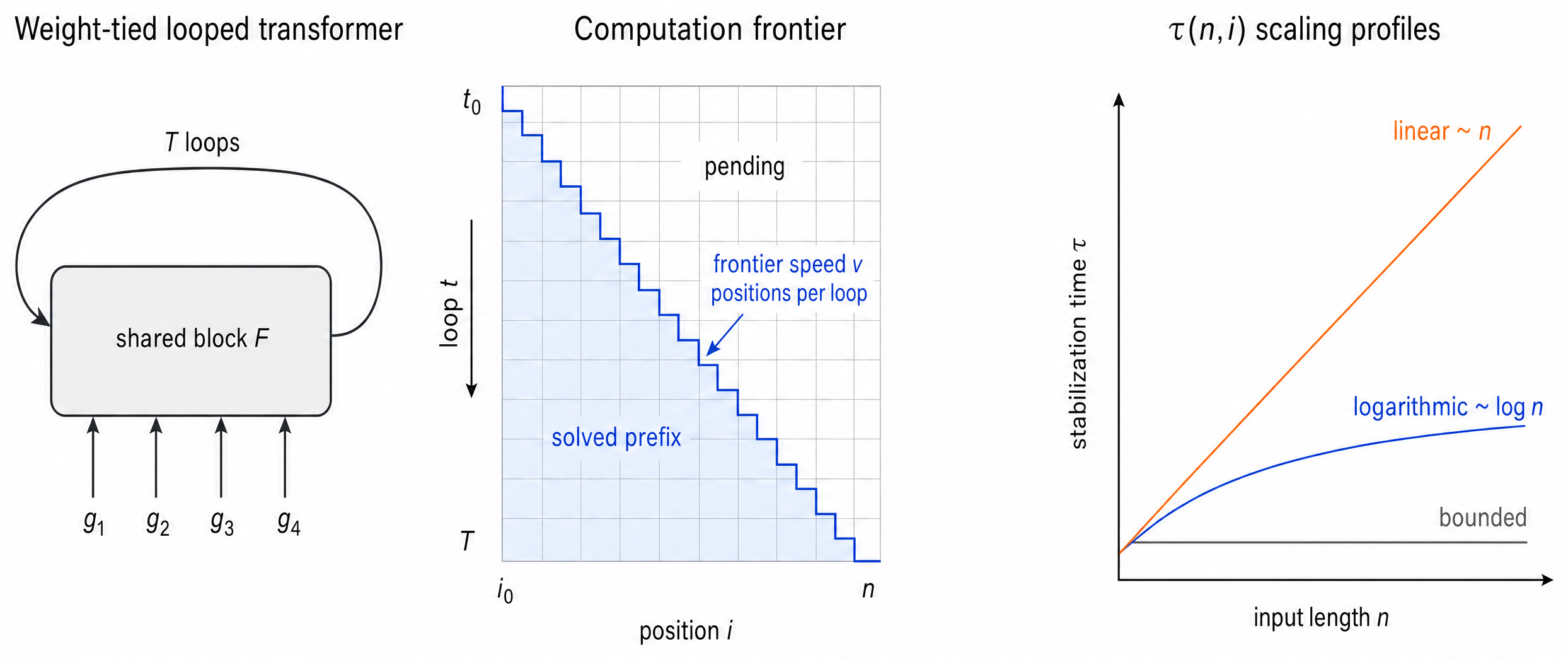
Our experiments reveal a visible pattern in many successful weight-tied models: a correct prefix moves through the input. Its leading edge is a computation frontier. Changing the loop allowance during training changes how quickly that frontier advances. The interesting question becomes concrete: how much progress does a shared update make, and when does giving it another turn stop helping?
A sequence with an answer at every position
Imagine a list of permutations. Each permutation rearranges a finite set of objects. The answer at the first position is the first permutation; the answer at the next position is the composition of the first two; later answers compose longer prefixes. The task is simple to specify, yet it offers several possible computational strategies. A model can carry a running product along the sequence, or combine partial products in a more parallel organization.
This setting gives us exact supervision throughout the input. We do not need a verbal explanation from the model to decide which prefix products are correct. After every completed recurrent update, we decode the answer at each supervised position. The resulting loop-by-position map becomes a record of computational progress.
Weight tying means that the update function is reused. It does not require the hidden state to remain the same, nor does it force one loop to correspond to one symbolic operation. The state carries the changing context in which the same parameters operate. That distinction is central: architectural repetition supplies an opportunity for iteration; the learned dynamics determine what iteration does.
Why the end of a trajectory can hide its beginning
Suppose a trajectory reaches an exact fixed point: applying the update again leaves its state unchanged. Skipping a subsequent update then changes nothing. Local derivatives are evaluated at the same state on every later loop. A deterministic instrument using only that state and its local derivative consequently gives the same reading after every additional update.
This is a measurement limitation with a precise scope. Such readings cannot uniquely recover the computation that preceded the fixed point. A model may have performed substantial work before entering this quiet tail. Conversely, an unchanged output label does not establish that the hidden state has reached a fixed point. We therefore keep hidden-state stationarity, output stabilization, and correctness separate.
Our instrument looks earlier. For each position, we record when its predicted label settles to the final recorded label and stays there through the observation horizon. To describe useful partial computation, we also track the longest contiguous prefix that is correct at each update. Isolated correct answers beyond an unreliable position do not extend that frontier.
Watching the frontier move
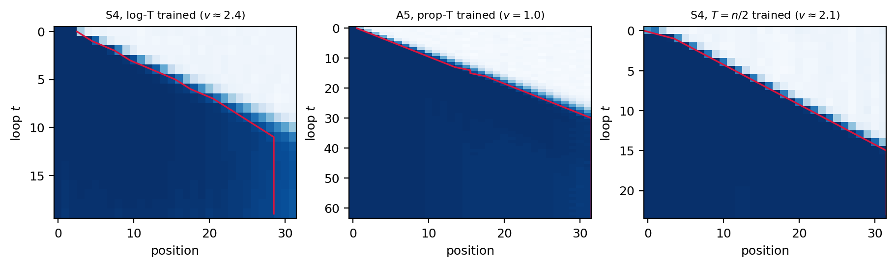
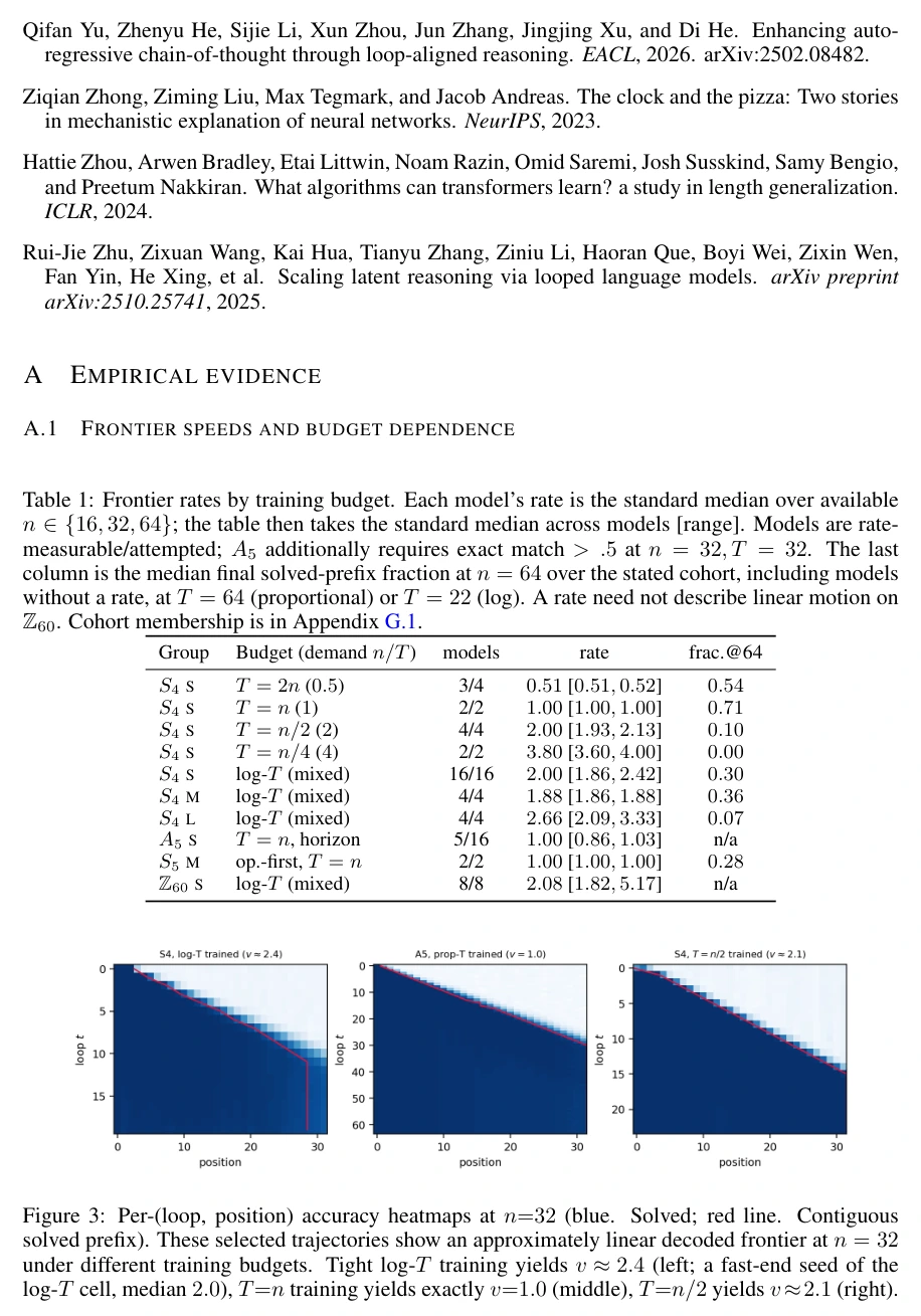
The heatmaps make an iterative procedure visible without claiming a unique internal circuit. Early positions become reliable before later ones. Across the measured lengths, many analyzed models extend the prefix at an approximately constant rate. Extra loops can move the boundary into positions that were previously wrong.
Frontier speed describes progress within a trajectory. Exact-match accuracy asks whether every required answer is correct. A model can have a measurable frontier and still fail the full task. If the frontier stalls halfway through a longer input, the model still fails the full task.
The same distinction matters for batch statistics. The frontier threshold is based on per-position batch accuracy. A region that is reliable across the batch need not imply that every individual sequence is solved. We retain competence measurements alongside the trajectory measurements rather than replacing them.
A training budget becomes pressure on each update
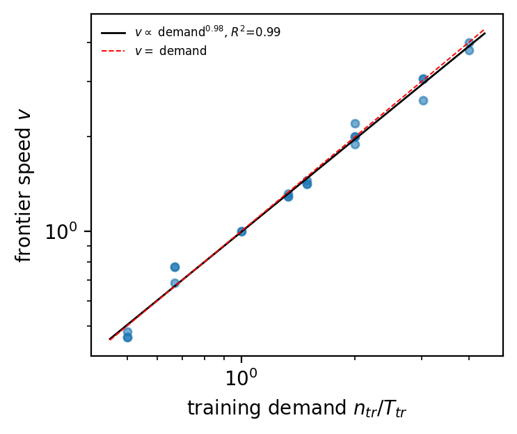
If training allows many loops for a sequence, each shared update can make relatively little progress and still finish in time. A tighter allowance demands that each update resolve more positions. We express this nominal demand as sequence length divided by the loop allowance. Proportional schedules keep that pressure approximately consistent as training sequences become longer; logarithmic schedules tighten it across stages.
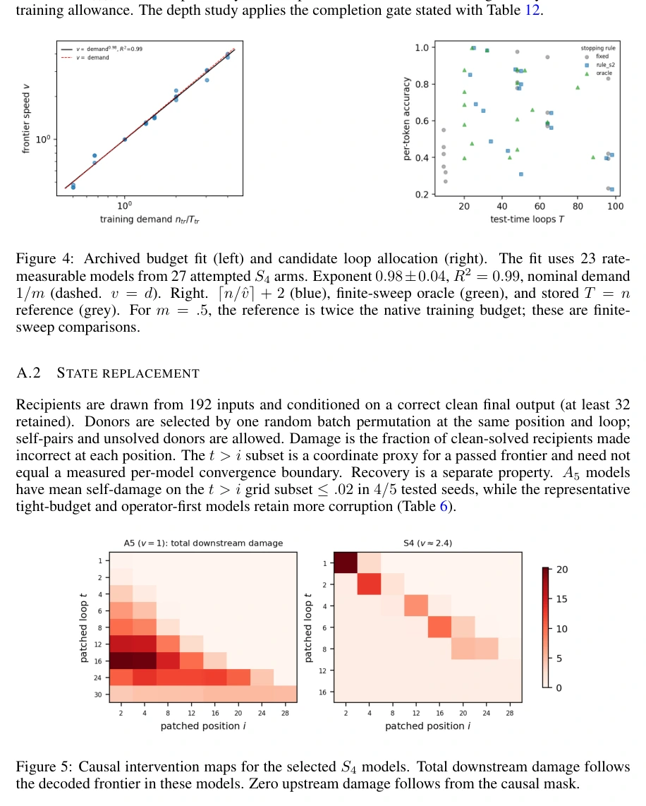
In the archived permutation-product sweep, 23 of 27 attempted S₄ arms have measurable frontier rates. Across the eligible demand range, the fitted exponent is 0.98 ± 0.04 with R² = 0.99. The near-unit exponent is the striking observation: measured progress per loop responds approximately proportionally to the demand imposed during training.
| S₄ training allowance | Nominal demand | Measurable / attempted | Median frontier rate |
|---|---|---|---|
| T = 2n | 0.5 | 3 / 4 | 0.51 |
| T = n | 1 | 2 / 2 | 1.00 |
| T = n / 2 | 2 | 4 / 4 | 2.00 |
| T = n / 4 | 4 | 2 / 2 | 3.80 |
The table reports the standard median rate across the available models, following the manuscript’s frontier-rate table. It is a compact view of the relation, not a claim that every trained run has a measurable linear trajectory. No rate from the three attempted T = 3n arms enters the archived fit. The result is an empirical relation in this measured S₄ population, not a theorem that optimization always selects a minimum-speed solution.
Intervening on the computation
A decoded pattern might be an informative readout without identifying the hidden states that matter to the answer. We therefore replace an intermediate state with a state from another input, continue the original recurrence, and measure damage to the final output.
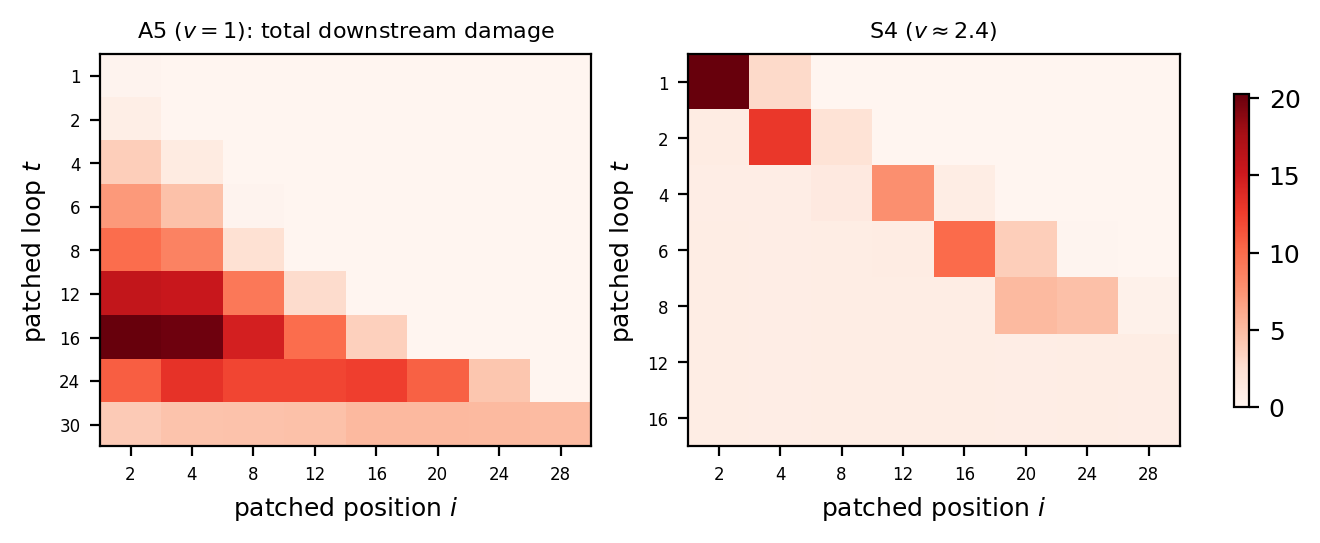
State replacement tests how changing an intermediate state changes the final answer. In the selected models, the damage boundary follows the organization suggested by the frontier. Recovery must still be measured separately: some models repair particular replacements, while others retain the corruption.
The intervention therefore supports frontier-organized dependencies for the models tested. It does not promote every observed straight boundary into a validated circuit. Keeping those two claims separate makes the experiment more useful: the readout locates a candidate process, and the intervention tests consequences of perturbing it.
Learning an operation is different from reusing it
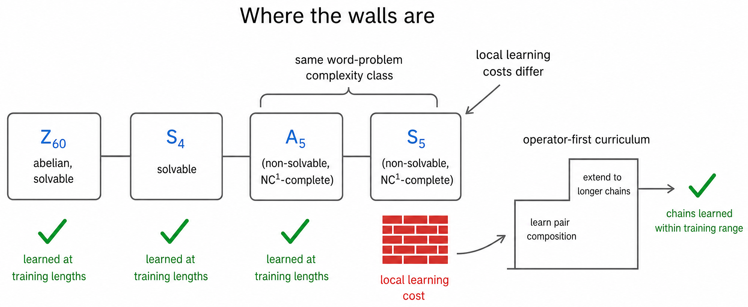
A prefix product requires both a local composition rule and a reliable way to apply it repeatedly. To separate these demands, we train an operator-first curriculum that emphasizes pair composition before extending to longer chains. This makes it possible to distinguish failure to learn the local operation from failure to organize or sustain its repeated use.
The S₅ operator-first setting learns chains within the training range more successfully than the compared free-training cohort. It does not establish successful length generalization. A frontier can continue advancing on longer inputs while exact-match accuracy stays low. Training steps and curriculum details also differ between cohorts, so the comparison does not isolate curriculum order alone.
Streaming input provides another control. Revealing successive tokens over successive loops constrains when an answer can become available. Parity learns under this schedule, while the tested difficult group tasks do not reach comparable competence. The release schedule calibrates timing under an explicit information constraint; it does not show that a freely presented sequence is processed by the same mechanism.
How much weight sharing is useful?
Recurrence is often contrasted with an entirely untied network, but that comparison combines several choices. We examine a ladder of weight-sharing degrees at fixed effective depth, both with fixed width and with parameter matching. Partial tying can outperform full tying, and the result changes with the parameter constraint.
The lesson is more specific than “recurrence wins.” Reusing weights is a useful architectural bias in these settings, but the most effective amount of sharing depends on the task and resource constraint. A mechanism claim should survive that distinction instead of borrowing strength from a single tied-versus-untied comparison.
Changing the allowance after training
Training separate models under different budgets shows an association. Budget transfer asks whether an existing model changes its trajectory when its allowance changes. Tightening the schedule accelerates measured frontiers in the tested group models, but that accelerated prefix can still fail to cover the complete sequence under the new allowance.
Relaxing the allowance can support successful training-length solutions while also producing slower measured frontiers. This separates adapting a partial computation from solving the target task. A checkpoint should therefore be measured again after transfer; its computational pace is not a permanent property inherited unchanged from its earlier training.
Another loop can help, and another can hurt
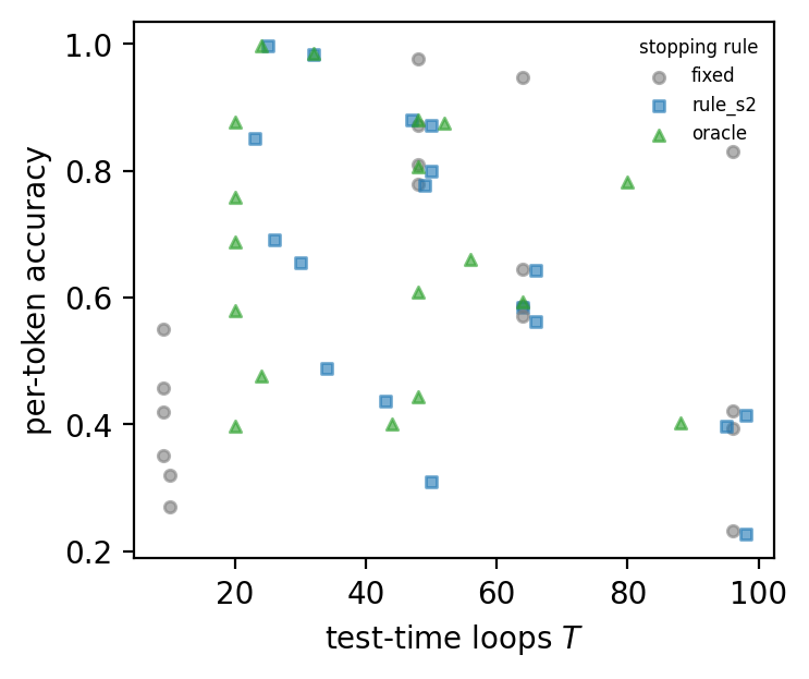
A frontier moving at a roughly constant speed suggests allocating enough loops to traverse the requested input, with slack for variation. This candidate rule can improve on stored schedule references for selected models. It estimates a sequence-level allowance from previous measurements; it does not detect per-input convergence online.
More loops are not an unconditional resource benefit. Before completion, an additional update may resolve a late position. After a correct answer appears, continued iteration may change it. Stalling also invalidates the extrapolation of a previously measured speed. This is why the trajectory, competence, and evaluation horizon must all be reported together.
What should we measure next?
Progress measurements at training lengths have task-dependent associations with longer-sequence accuracy. Frontier speed and completion associate positively with generalization in the evaluated group-task pairs; parity behaves differently. Similarity-based measurements also carry information, and the direction of an association can reverse across settings. A deployed predictor must fix its direction and selection rule before testing new models.
The central result is a way to connect a training choice to observable computation. Instead of treating every extra recurrent update as an anonymous unit of test-time compute, we can ask where it advances the answer, what hidden-state changes matter, whether the local operation is learned, and whether progress survives longer inputs. Those questions turn a repeated block into a measurable dynamical process.
Experimental record
The original result views below remain available alongside the expanded account. Figures and the compact rate table above are taken from the paper’s archived experiments and the local revised manuscript. This article introduces no new experimental runs.
Experimental results
Citation
@misc{zhang2026recurrentcircuits,
  title = {When Does Recurrence Become an Algorithm? Convergence Selection in Weight-Tied Looped Transformers},
  author = {Zhang, Tong and Hu, Junhao and Peng, Yun and Xie, Tao},
  year = {2026},
  eprint = {2607.20594},
  archivePrefix = {arXiv},
  primaryClass = {cs.LG},
  url = {https://arxiv.org/abs/2607.20594}
}